Understanding the Crystal Ball Function

Exploring the intricacies of the Crystal Ball Problem as it applies to arrays, this piece delves into the challenge of predicting future elements based on current sequences. It underscores the significance of pattern recognition and algorithmic forecasting in computational analysis and real-world applications.

Introduction

The Crystal Ball Problem is a metaphor for predicting future elements or trends in an array based solely on its current sequence. Imagine you have an array of numbers representing data points over time—such as stock prices or weather data—and your task is to forecast the upcoming values. The “crystal ball” is our metaphor for the ability to foresee these future values.

In computational terms, this problem relates to creating algorithms that analyze and extrapolate patterns from arrays. Given an array $A$ of length $n$ with elements

$$A[1], A[2], \dots, A[n],$$

the challenge is to predict

$$A[n+1], A[n+2], \dots$$

based on the underlying patterns or rules governing the progression of the array’s elements.

Why Square Root of n?

Optimization Balance

When using Jump Search in a sorted array, the search is divided into two phases:

1. Jump Phase: Jump in fixed blocks until you find a block that may contain the target.
2. Linear Search Phase: Perform a linear search within that block.

The total number of steps can be roughly modeled as the sum of the number of jumps and the number of steps in the linear search. By choosing a block size $m$ proportional to $\sqrt{n}$, we optimize this sum.

Trade-off Between Jump and Search

• Large Jump Size (e.g., using $n^{1/3}$): Fewer jumps but a longer linear search.
• Small Jump Size (less than $\sqrt{n}$): More jumps but a shorter linear search.

The square root of $n$ balances the two phases so that neither dominates the total search time.

Theoretical Justification

Mathematically, when you differentiate the total search steps with respect to $m$ and set the derivative to zero, you find that the optimal $m$ is proportional to $\sqrt{n}$. This balance minimizes the worst-case scenario search time.

Alternative Roots

Using an alternative root such as the cube root of $n$ would disturb this balance. It might reduce the number of jumps but at the expense of increasing the number of elements checked in the linear search phase—or vice versa. The square root remains the most effective choice in general because it equally balances both components of the search.

Mathematical Justification

Setting Up the Problem

In Jump Search, you jump through an ordered list in increments of $m$ until you overshoot the target value. Then, you perform a linear search in the identified block. The key is to minimize the total number of steps.

• Maximum number of jumps: $\frac{n}{m}$
• Maximum number of linear search steps: $m - 1$ (or simply $m$ for simplicity)

Thus, the total number of steps $T(m)$ can be approximated by:

$$T(m) = \frac{n}{m} + m.$$

Total Search Steps

The function

$$T(m) = \frac{n}{m} + m$$

captures the trade-off: decreasing $m$ increases the jump count, while increasing $m$ lengthens the linear search.

Finding the Optimal m

To find the optimal block size $m$, differentiate $T(m)$ with respect to $m$:

$$\frac{d}{dm}T(m) = -\frac{n}{m^2} + 1.$$

Setting the derivative to zero gives:

$$-\frac{n}{m^2} + 1 = 0 \quad \Longrightarrow \quad m^2 = n,$$

which implies:

$$m = \sqrt{n}.$$

Example with n = 100

For an array of 100 elements:

$$m = \sqrt{100} = 10.$$

This means:

• Jump Size: Jump every 10 elements (i.e., indices 0, 10, 20, …, 90).
• Linear Search: After jumping, perform a linear search in a block of up to 10 elements.

Illustration with Python Code

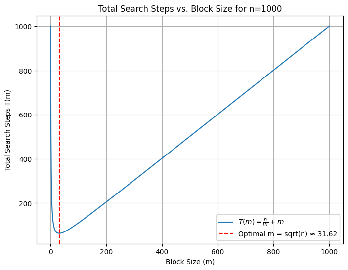
Below is a Python code snippet that plots the total search steps $T(m)$ against different block sizes $m$ for a given $n$. The plot highlights the optimal block size at $m = \sqrt{n}$.

import matplotlib.pyplot as plt
import numpy as np

# Set array length
n = 1000

# Generate a range of possible m values
m_values = np.linspace(1, n, 1000)
T = n / m_values + m_values

# Calculate optimal m
optimal_m = np.sqrt(n)

# Plot the total search steps vs. block size
plt.figure(figsize=(8, 6))
plt.plot(m_values, T, label=r'$T(m)=\frac{n}{m}+m$')
plt.xlabel('Block Size (m)')
plt.ylabel('Total Search Steps T(m)')
plt.title(f'Total Search Steps vs. Block Size for n={n}')
plt.axvline(x=optimal_m, color='red', linestyle='--', label=f'Optimal m = sqrt(n) ≈ {optimal_m:.2f}')
plt.legend()
plt.grid(True)
plt.show()

Explanation:
The code above computes and plots $T(m)$ for $n = 1000$ over a range of $m$ values. The vertical dashed line indicates the optimal block size $m = \sqrt{1000}$.

Conclusion

The use of $m = \sqrt{n}$ in the Jump Search algorithm optimally balances the number of jumps and the linear search steps, leading to a worst-case time complexity of $O(\sqrt{n})$. This balance is crucial for efficient search in unsorted or partially ordered arrays, and the mathematical justification confirms the effectiveness of this approach.