This cheat sheet is based on “Heliospheric Coordinate Systems” by Franz & Harper (2002, corrected 2017). It’s written for readers comfortable with high-school algebra, geometry, trigonometry, and a bit of Calculus I.

1. Big Picture

In space science, we constantly answer questions like:

Where is this planet or spacecraft right now?
How do its coordinates in one system (e.g. Earth-centered) translate to another (e.g. Sun-centered)?
How do we describe an orbit in a compact, reusable way?

To do that, we need:

Coordinate systems – ways to define X, Y, Z in space.
Time systems – to know when we’re measuring things.
Keplerian orbital elements – six numbers that define the shape and orientation of an orbit.

This page is a “translation layer” between the formal paper and a beginner-friendly reference.

2. Angles, Directions, and Basic Terms

2.1 Right Ascension (RA, `α`) and Declination (Dec, `δ`)

These are like longitude and latitude projected onto the sky.

Right Ascension (α)
- Measured along the celestial equator (Earth’s equator extended into space).
- Units: hours, minutes, seconds (0–24 hours).
- 24h = 360°, so 1h = 15°.
Declination (δ)
- Measured north/south of the celestial equator.
- Units: degrees (−90° to +90°).
- +90° is the North celestial pole; −90° is the South celestial pole.

Think:
RA/Dec are “coordinates on the dome of the sky.”

2.2 Ecliptic and Obliquity (`ε`)

Ecliptic plane
- The plane of Earth’s orbit around the Sun.
- Used as a natural reference plane for the solar system.
Obliquity of the ecliptic (ε)
- Angle between Earth’s equatorial plane and the ecliptic.
- About 23.44° today.

So:

Equatorial coordinates use Earth’s equator.
Ecliptic coordinates use Earth’s orbital plane.

The tilt between these is ε.

3. Coordinate Systems (Conceptual Overview)

We’ll use these labels:

GEI – Geocentric Earth Inertial (Earth-centered, equator of J2000)
GEO – Geographic (latitude/longitude on Earth’s surface)
HAE – Heliocentric Aries Ecliptic (Sun-centered, Earth’s orbital plane)
HEE / GSE / GSM / SM / MAG – special systems used for space physics

We won’t go into every niche system, but we’ll give you the mental picture.

3.1 Geocentric Earth Equatorial (GEI, aka GEI J2000)

Origin: Earth’s center
XY-plane: Earth’s equatorial plane at epoch J2000.0
+Z: points to the North celestial pole
+X: points towards the vernal equinox (the direction of the Sun at March equinox)

This is a “fixed” inertial frame used for star positions and high-precision work.

3.2 Heliocentric Aries Ecliptic (HAE J2000)

Origin: Sun
XY-plane: Earth’s ecliptic plane at J2000.0
+Z: ecliptic north
+X: toward the vernal equinox

This is the natural frame for planetary orbits and is what the Keplerian elements in the paper use.

3.3 Common Solar–Terrestrial Systems (High Level Only)

These appear often in space physics:

HEE (Heliocentric Earth Ecliptic)
- Sun at origin, XY-plane = ecliptic.
- +X points from Sun to Earth.
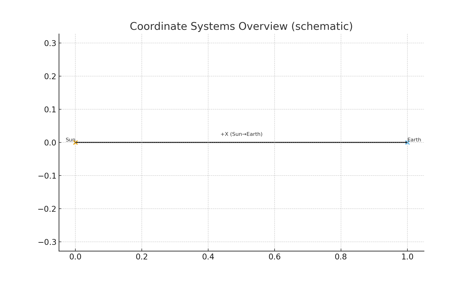
GSE (Geocentric Solar Ecliptic)
- Earth at origin, XY-plane = ecliptic.
- +X points from Earth to Sun.
GSM (Geocentric Solar Magnetospheric)
- Earth at origin.
- +X toward Sun, +Z aligned with Earth’s magnetic dipole (projected appropriately).
SM, MAG, etc.
- Variations that align Z with Earth’s magnetic pole, etc.

You don’t need every detail; just remember each system chooses:

An origin (Earth, Sun, spacecraft)
A reference plane (equator, ecliptic, solar equator)
A direction for +X (Sun, equinox, magnetic pole, etc.)

4. Euler Rotation Matrices (Concept Only)

To go from one coordinate system to another, the paper uses Euler rotations, denoted:

E(Ω, θ, φ)

Meaning:

Rotate about Z by Ω
Rotate about X by θ
Rotate about Z by φ

Mathematically, it’s a 3×3 matrix that you multiply your vector by:

r_new = E(Ω, θ, φ) · r_old

For example, to go from equatorial to ecliptic coordinates at J2000, a simple rotation by the obliquity ε is:

E(0, ε, 0)

You don’t need to memorize the whole matrix; just remember:
Euler angles = a systematic way to describe 3D rotations.

5. Keplerian Orbital Elements – Definitions for Beginners

An orbit (around the Sun, a planet, etc.) can be described by six numbers.

For a body orbiting the Sun (heliocentric orbit):

Semi-major axis (a)
Eccentricity (e)
Inclination (i)
Longitude of ascending node (Ω)
Argument of periapsis (ω)
Mean anomaly at epoch, or time of periapsis passage (M₀ or T)

We’ll unpack each.

5.1 Semi-Major Axis (`a`)

Half of the longest diameter of the ellipse.
Sets the overall size of the orbit.
Units: usually AU (astronomical units) for planetary orbits.

Example:
Earth’s orbit has a ≈ 1 AU, Mars has a ≈ 1.52 AU.

5.2 Eccentricity (`e`)

Measures how stretched the ellipse is.
e = 0 → perfect circle
0 < e < 1 → ellipse
e = 1 → parabola (escape)
e > 1 → hyperbola (flyby / escape trajectory)

Example:
Earth: e ≈ 0.0167 (almost circular)
Mars: e ≈ 0.093 (slightly more oval)

5.3 Inclination (`i`)

Tilt of the orbital plane relative to a reference plane (e.g. ecliptic).
Measured in degrees (0°–180°).
i = 0°: orbit lies in the reference plane.

5.4 Longitude of Ascending Node (`Ω`)

Where the orbital plane crosses the reference plane going south → north.

The ascending node is that crossing point.
Ω is the angle (in the reference plane) from a fixed direction (usually the vernal equinox) to the ascending node.

Think:
“You stand at the Sun and look at the orbital plane: Ω tells you where the orbit intersects the reference plane going upward.”

5.5 Argument of Periapsis (`ω`)

Once you’re in the orbital plane:

ω is the angle from the ascending node to periapsis (closest point to the Sun), measured along the orbit.

So:

Ω locates the orbital plane and node in space.
ω locates periapsis inside that plane.

5.6 True Anomaly (`ν`)

Angle from periapsis to the current position along the orbit, measured at the focus.
Changes non-linearly with time: object moves faster near periapsis and slower near apoapsis.

5.7 Mean Anomaly (`M`) and Mean Motion (`n`)

Kepler’s second law (equal areas in equal times) makes ν change irregularly in time. To simplify:

Mean motion:
n = 2π / P
where P is the orbital period.
Mean anomaly (M):
Angle that increases uniformly in time:
```
M(t) = n (t − T)
```
where T is the time of periapsis passage.

So:

M is a “clock angle” – easy to integrate in time.
We later convert M → E → ν.

5.8 Eccentric Anomaly (`E`)

A helper angle used to relate mean anomaly M to true anomaly ν for an elliptical orbit.

For an ellipse:

M = E − e sin E        (Kepler’s equation, elliptic case)

This equation cannot be solved algebraically for E; we use iteration (e.g. Newton’s method).

6. From Orbital Elements to Position – Step-by-Step

We want to go from orbital elements to an actual 3D position vector r = (x, y, z) in some frame (e.g. heliocentric ecliptic).

Given:

a, e, i, Ω, ω
M(t) at the time of interest (or T, then compute M)

We do:

Compute M at time t
Solve Kepler’s equation for E
Convert E → ν
Compute radial distance r
Compute position in the orbital plane (perifocal frame)
Rotate into the chosen inertial frame with Euler rotations

6.1 Step 1 – Mean Anomaly at Time `t`

If you know:

M₀ at epoch t₀
Mean motion n

Then:

M(t) = M₀ + n (t − t₀)

Or if you know time of periapsis T:

M(t) = n (t − T)

6.2 Step 2 – Solve Kepler’s Equation for E

For an elliptical orbit (0 < e < 1):

M = E − e sin E

We solve for E by iteration. Using Newton’s method:

E_{k+1} = E_k − (E_k − e sin E_k − M) / (1 − e cos E_k)

A good first guess is E₀ = M (if e is small).

Worked Example (Kepler’s Equation Only)

Suppose:

e = 0.1
M = 1.0 rad (about 57.3°)

Initial guess: E₀ = 1.0
Plug into Newton’s method:
```
f(E)   = E − e sin E − M
f'(E)  = 1 − e cos E
```
Compute with a calculator or code; after a couple of iterations, E will converge (typically within 2–4 steps).

6.3 Step 3 – Convert `E → ν` (True Anomaly)

We can use:

cos ν = (cos E − e) / (1 − e cos E)
sin ν = (sqrt(1 − e²) sin E) / (1 − e cos E)

Then ν = atan2(sin ν, cos ν).

6.4 Step 4 – Radial Distance `r`

Either:

r = a (1 − e cos E)

r = p / (1 + e cos ν)
where p = a (1 − e²)

Both are equivalent.

6.5 Step 5 – Position in the Perifocal Frame

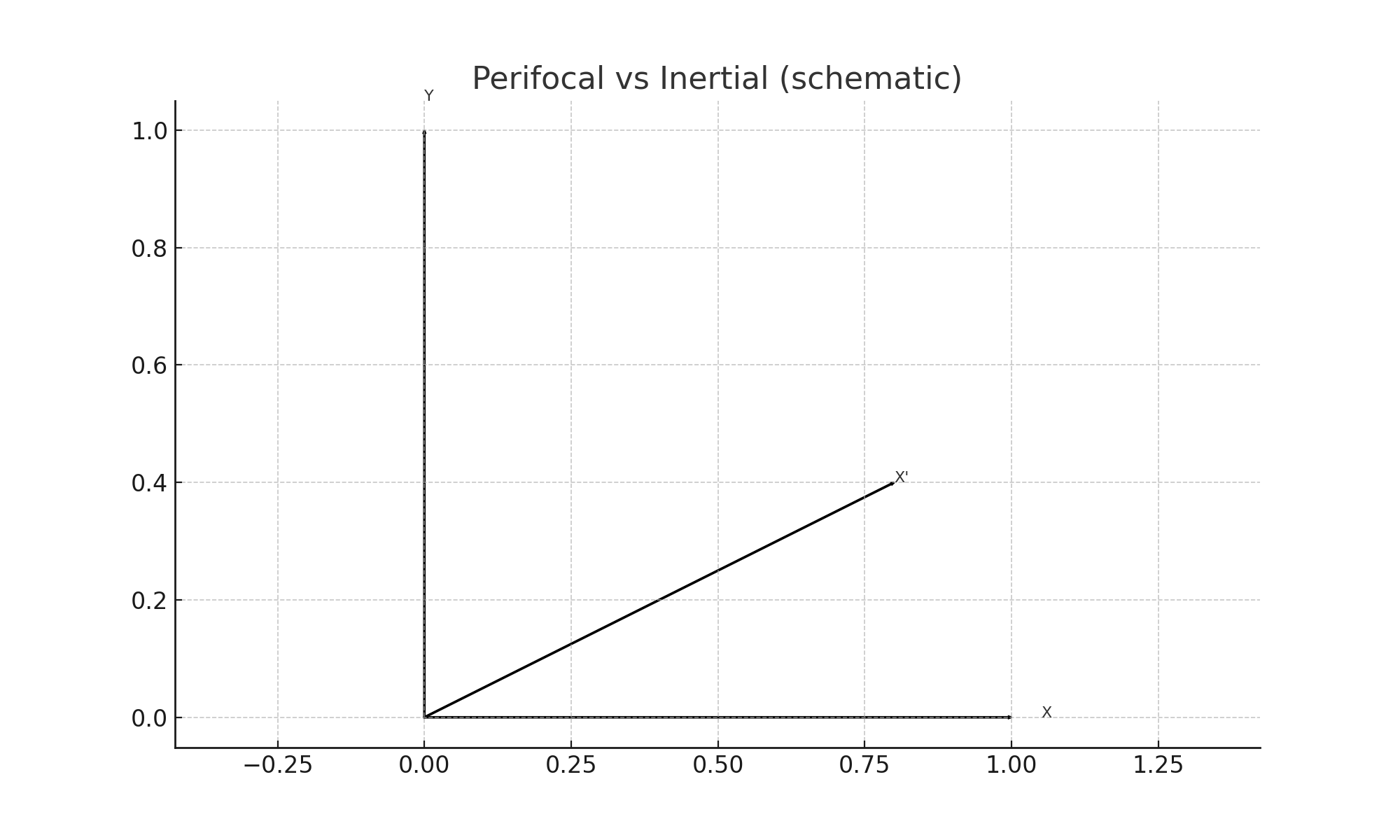
The perifocal frame is:

Origin: central body (e.g. Sun)
+X’ axis: points toward periapsis
+Y’ axis: 90° forward along direction of motion
+Z’ axis: perpendicular to orbital plane (right-hand rule)

In this frame:

r_perif = [ r cos ν,
            r sin ν,
            0           ]

Velocity (if desired):

v_perif = sqrt(μ / p) [ −sin ν,
                        e + cos ν,
                        0           ]

Where:

μ = GM of central body (e.g. Sun)
p = a (1 − e²)

6.6 Step 6 – Rotate Into Heliocentric Ecliptic (HAE)

To go from perifocal coordinates to a standard inertial frame (like HAE J2000), we use Euler rotations with the orbital angles:

r_inertial = R(Ω, i, ω) · r_perif

Where R(Ω, i, ω) is equivalent to the Euler sequence:

E(Ω, i, ω)

Conceptually, this:

Rotates the orbital plane by ω around Z'
Tilts by inclination i
Spins around the reference Z by Ω to match the ascending node

In practice, you’d plug numbers into the rotation matrix or use a library.

7. A Simple Toy Orbit Example (All Steps)

Let’s create a fake planet with:

a = 1 AU
e = 0.1
i = 5°
Ω = 30°
ω = 45°
At epoch t₀, let M₀ = 10° (≈ 0.1745 rad)

Suppose we want position at t = t₀ (just to keep it simple):

Compute M at t
- M = M₀ = 0.1745 rad.
Solve Kepler’s equation M = E − e sin E
- Start with E₀ = M = 0.1745.
- Apply Newton iterations until E converges (you’d use code or a calculator).
Find ν from E
- Use the formulas above for cos ν and sin ν, then ν = atan2.
Compute r
- r = a (1 − e cos E).
Perifocal position
- r_perif = [r cos ν, r sin ν, 0].
Rotate to inertial
- Convert angles to radians:
  - i = 5°, Ω = 30°, ω = 45°.
- Build rotation matrix R(Ω, i, ω).
- Compute r_inertial = R · r_perif.

You don’t need to do all arithmetic by hand; this sequence is what software implements.

8. Diagrams

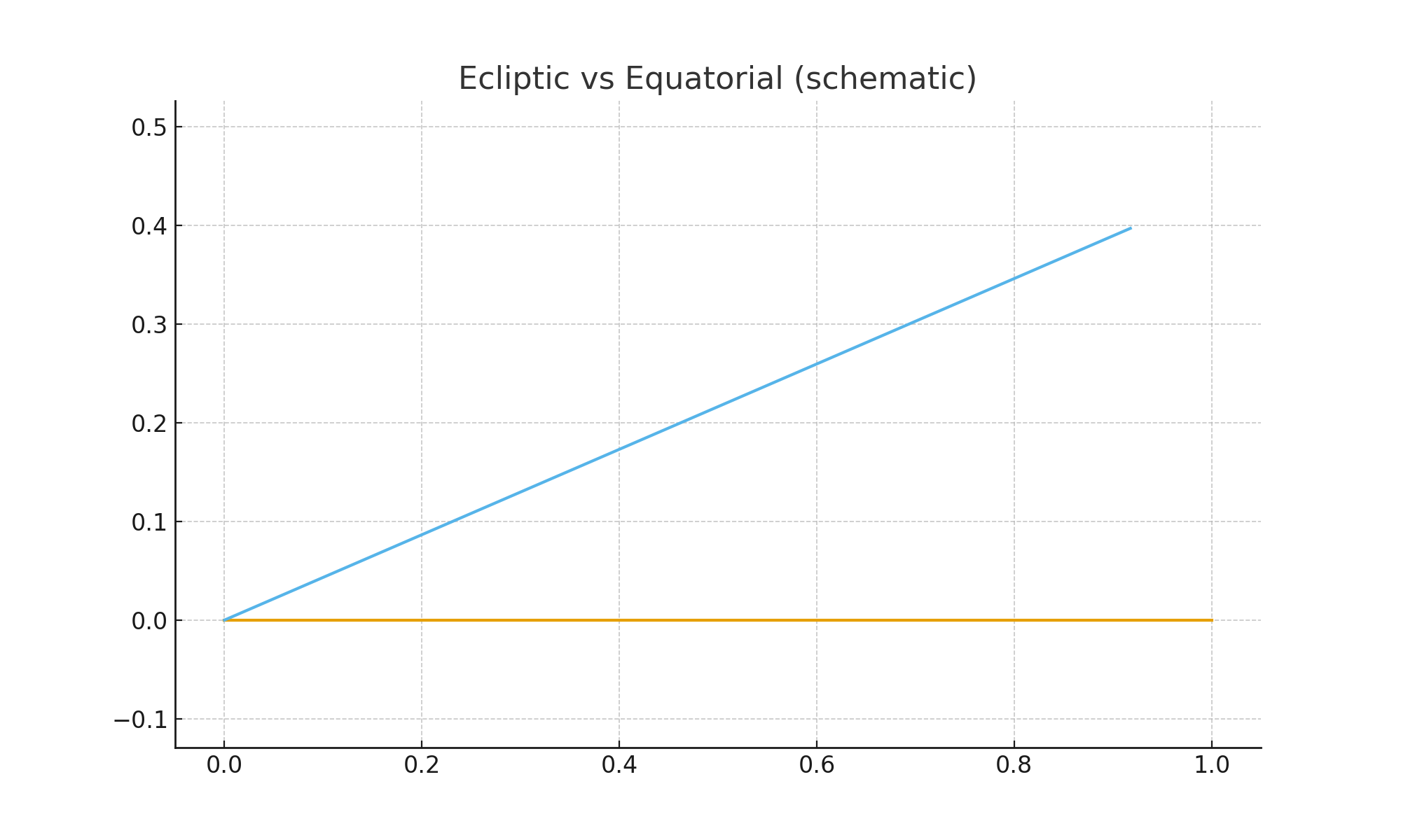
8.1 Ecliptic vs Equatorial Planes

Ecliptic vs Equatorial Planes

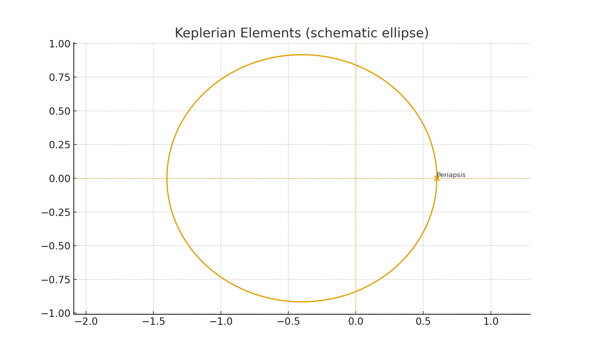
8.2 Keplerian Elements Geometry

Keplerian Orbital Elements

8.3 Perifocal vs Inertial Frames

Perifocal vs Inertial Frames

8.4 Simple Coordinate System Comparison

Coordinate Systems Overview

9. Common Symbols & Constants

A quick reference.

μ – gravitational parameter = G × (central mass)
μ_⊙ ≈ 1.3271244 × 10¹¹ km³/s² (Sun)
a – semi-major axis
e – eccentricity
i – inclination
Ω – longitude of ascending node
ω – argument of periapsis
ν – true anomaly
E – eccentric anomaly
M – mean anomaly
P – orbital period
n = 2π / P – mean motion
AU ≈ 1.49597870 × 10⁸ km – astronomical unit
k = 0.01720209895 – Gaussian gravitational constant

10. How to Use This Cheat Sheet

Use Sections 5–7 when you want to go from orbital elements to a physical position.
Use Sections 2–3 & 8 when translating between different coordinate systems and visualizing geometry.
Use Section 9 as a quick reference for symbols.

You can expand this page into multiple Hugo pages later (e.g. “Basics”, “Orbits”, “Coordinate Systems”), but this single markdown file is a good starting point.

Heliospheric Coordinate Systems & Keplerian Orbits – Beginner Cheat Sheet